Abstraction: Thinking at the Right Level

A program can be understood at many levels. We might ask what a function computes, how its data is represented, which instructions a compiler produces, or how a processor executes them. Each question reveals something useful, but trying to answer all of them at once quickly becomes overwhelming.

Abstraction gives us a way to choose. We describe the behavior that matters at one level and put other details behind an interface. This article follows that idea from small Python functions down through the layers of a computer.

Part I: Abstraction in Programs

Naming a process

A useful starting point is to see a program as data and procedures that operate on it:

scores = [82, 95, 71]  # data
scores.sort()         # a procedure acting on that data

Data answers “What are we working with?” A procedure answers “What do we do with it?”

Consider the expression 3 * 3 + 4 * 4. The same pattern appears twice: multiply a number by itself. We can give that pattern a name:

def square(x):
    return x * x

square(3) + square(4)  # 25

This is procedural abstraction. A concrete sequence of operations becomes a reusable part of our vocabulary. Once we understand what square does, we can reason about the expression using that meaning.

Separating data from its representation

Suppose we want to represent rational numbers while keeping their numerators and denominators. We begin with three operations:

• rational(n, d) constructs the rational number n/d.
• numer(r) returns its numerator.
• denom(r) returns its denominator.

The numerator and denominator are integers, and the denominator must be nonzero. Using the familiar rule a/b + c/d = (ad + bc)/(bd), we can write addition before choosing a storage format:

def add_rational(x, y):
    n = numer(x) * denom(y) + numer(y) * denom(x)
    d = denom(x) * denom(y)
    return rational(n, d)

One implementation uses lists:

def rational(n, d): return [n, d]
def numer(r): return r[0]
def denom(r): return r[1]

Another uses dictionaries:

def rational(n, d): return {"n": n, "d": d}
def numer(r): return r["n"]
def denom(r): return r["d"]

These minimal examples assume valid inputs and omit fraction reduction. With either implementation, adding 1/2 and 1/3 produces a rational number with numerator 5 and denominator 6.

The important detail is what add_rational never asks: whether its arguments contain list indices or dictionary keys. It depends only on the three agreed operations.

That interface forms an abstraction barrier between arithmetic and representation. If we replace the representation and update its operations together, the arithmetic code can stay the same. Directly accessing x[0] inside add_rational would cross that barrier and couple addition to the list implementation.

Treating functions as data

The distinction between data and procedures becomes more interesting when procedures themselves can be values:

operation = square
operation(3)  # 9

In Python, functions can be assigned names, passed as arguments, and returned as results. This lets us abstract over recurring patterns of computation.

To square every number in a sequence, we could write:

xs = [1, 2, 3]
results = []
for x in xs:
    results.append(square(x))

The pattern is “take each element, apply an operation, collect the results.” map captures the application step:

list(map(square, xs))  # [1, 4, 9]

Here, square specifies how to transform an element, while xs supplies the elements. list collects the results from the iterator returned by map.

There is a crucial difference between square and square(3): the first is a function; the second is the result of calling it. Passing a function gives another procedure a computation it can perform later, on its own inputs.

Changing that function changes the transformation without changing the surrounding pattern:

def double(x):
    return 2 * x

list(map(square, [1, 2, 3]))  # [1, 4, 9]
list(map(double, [1, 2, 3]))  # [2, 4, 6]

Building functions out of functions

We can go further: a function can accept existing functions and construct a new one. Parser combinators offer a concrete example.

A small parser recognizes something simple, such as an integer or a symbol. Combinators assemble those parsers into larger ones. The following is a teaching sketch using the vocabulary of my py-parser project; it assumes the parser primitives and arithmetic operators are already defined:

number = token(integer)
bracketed = between(
    symbol("("), lazy(lambda: expr), symbol(")")
)
times = fmap(symbol("*"), lambda _: mul)

atom = choice(number, bracketed)
term = chain_left(atom, times)
expr = chain_left(term, choice(plus, minus))

parse(expr, "2 + 3 * (4 - 1)")  # 11

An atom is either a number or a parenthesized expression. A term chains atoms with multiplication. An expression chains terms with addition or subtraction. This structure expresses operator precedence: multiplication is grouped inside the terms that addition and subtraction combine. lazy delays access to expr, allowing parentheses to refer back to the expression parser.

At this level, we can think in terms of grammatical rules. The combinators handle the repeated mechanics of combining parsers. The arithmetic evaluator built with this approach also supports division and unary signs:

from arith_evaluator import evaluate

evaluate("-(2 + 3) * 4 / 2")  # -10.0

This illustrates a central idea in functional programming: construct programs through function application and composition. Procedural programming emphasizes sequences of steps organized into procedures. Both provide useful ways to structure a computation, and the same program can use both.

Treating programs as data

The same parser vocabulary—operations such as choice, between, many, and lazy—can describe a small Lisp. Parsing an expression first produces a data structure:

from lisp_evaluator import parse_expression

parse_expression("(+ 2 (* 3 4))")
# ['+', 2, ['*', 3, 4]]

An evaluator can then interpret that structure. Lisp makes the connection between expressions and data particularly visible:

lisp> (+ 2 (* 3 4))
14
lisp> '(+ 2 (* 3 4))
(+ 2 (* 3 4))

The quote preserves the expression as data instead of evaluating it. With function definitions, our small language gains its own procedural abstractions:

lisp> (define square (lambda (x) (* x x)))
<procedure>
lisp> (square 7)
49

The Mini Lisp REPL repeatedly reads input, parses it, evaluates it, and prints the result. We have moved from naming a multiplication in Python to building a language in which someone else can name their own computations.

Part II: Abstraction Across the Computer

Source code and machine instructions

A high-level program specifies a computation. Different instruction sequences can implement it.

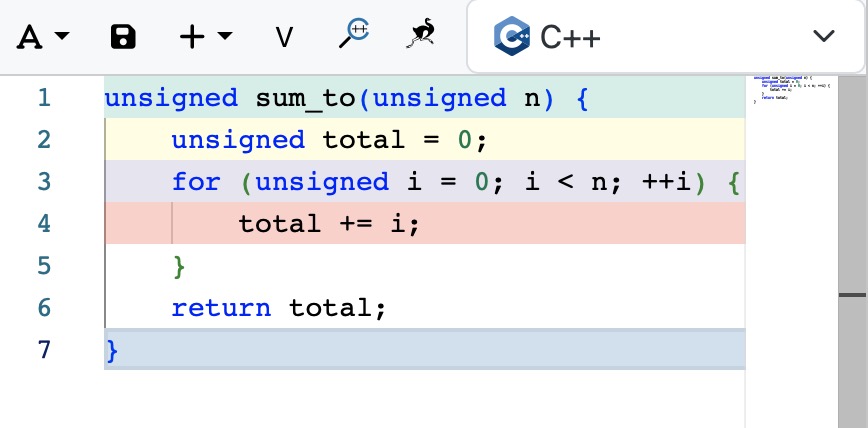
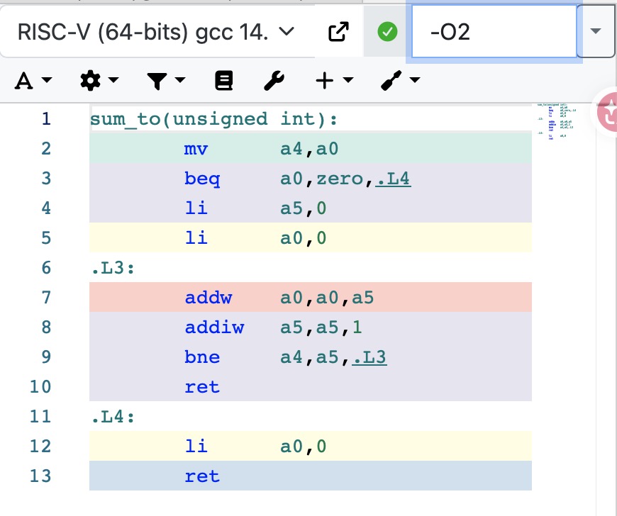
The same source produces a loop in the GCC example and an arithmetic calculation in the Clang example:

GCC · RISC-V 64-bit · O2	Clang · RISC-V 32-bit · O2

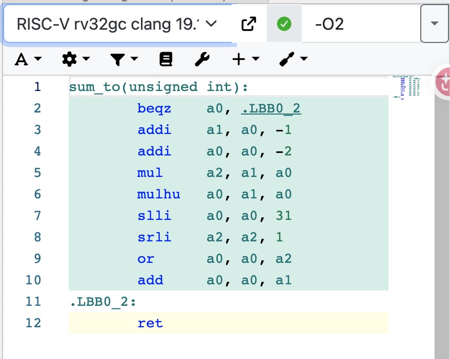These particular compilations illustrate implementation freedom within the source language’s rules. Results depend on compiler version, target, and options. Click either image to inspect it at full size.

Instructions and their execution

The instruction set defines operations and their effects. The processor decides how to schedule them, subject to dependencies:

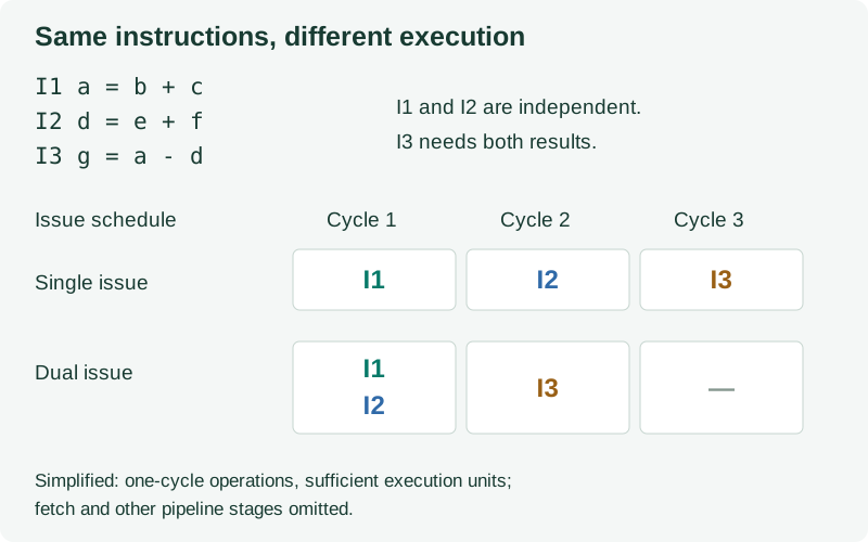
The same instructions can therefore run differently on different microarchitectures.

Pointers, memory, and operating systems

Abstraction	What it lets us reason about
Pointer	An allocation and an offset, beyond just numeric address bits
Virtual memory	A process’s address space, with physical mappings managed underneath
Processes and threads	Execution contexts, with processor time distributed by a scheduler

For pointer semantics, see Pointers Are Complicated, or: What’s in a Byte?. For memory and concurrency, start with the OSTEP introduction.

The useful skill is knowing when to change levels: arithmetic when adding fractions, representation when changing storage, and lower layers when investigating performance or system behavior.

Appendix: Courses, Projects, and Further Reading

Courses

• CS61A — Practice constructing, combining, and interpreting programs. Its treatment of abstraction connects many of the ideas above. The Fall 2024 archive is another reference.
• CS50x — A possible starting point for readers completely new to programming.
• CS61B — Continue with data structures, algorithms, and software engineering fundamentals.
• CS61C — Explore how programs run on machines.

More places to explore

• CS自学指南 / csdiy
• 帆影 on Bilibili
• Tsoding Daily and Tsoding’s main channel
• matklad’s blog and Fantastic Learning Resources